Abstract

Ocean heat transport near the tropical/subtropical boundary of the North Pacific during 1993-1998 is described, including its mean and time variability. Twenty-five transpacific high resolution XBT/XCTD transects (Fig. 1) are used together with directly measured and operational wind estimates to calculate the geostrophic and Ekman transports. The mean heat transport across the XBT transect is 0.77 ± 0.12 pW. The large number of transects enables a stable estimate of the mean field with realistic error bars based on the known variability. The North Pacific heat engine is a shallow meridional overturning circulation that includes warm Ekman and western boundary current components flowing northward, balanced by southward flow of cool thermocline waters (including Subtropical Mode Waters). A near-balance of geostrophic and Ekman transports holds in an interannual sense as well as for the time mean. The interannual range in heat transport was about 0.3 pW during 1993-1998, with maximum values of about 1 pW in early 1994 and early 1997. The repeating nature of the XBT/XCTD transects, with direct wind measurements, allows a substantial improvement over previous heat transport estimates based on one-time transects. A global system is envisioned for observing the time-varying ocean heat transport and its possible feedback in the coupled climate system.

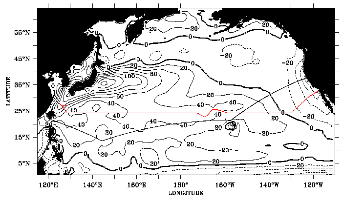
Figure 1. The PX37/10/44 ship track (solid line from San Francisco to Honolulu to Guam to Taiwan) is shown together with the ship track from the 24°N hydrographic transect (black line), and ECMWF air-sea heat flux (w/m2) averaged over the period 1993-1998. Positive numbers indicate heat loss by the ocean. The red line shows the ship track from the WOCE 24 N CTD section.

1. Introduction

The surplus of solar heating in the tropics and the corresponding deficit in polar regions gives rise to time-varying atmospheric and oceanic circulations that carry enormous amounts of heat poleward from the low latitudes. Measurements of the Earth's radiation budget (Stephens et al, 1981, Trenberth and Solomon, 1994) indicate that about 5 pW is carried northward across 24°N by the combined atmosphere and oceans. Estimates of the oceanic component, based on either oceanic measurements (Bryden et al, 1991) or on the residual of atmospheric transport and top-of-atmosphere radiation budgets (Trenberth and Solomon, 1994), have converged to about 2 pW at 24°N. However, the combined and individual estimates for ocean basins still have very large errors - 0.3 pW or greater. An improved understanding of the coupled climate system requires that the atmospheric and oceanic contributions to the planetary heat balance be known with better accuracy than at present. Further, it is necessary to investigate the low frequency variability of the coupled system. If there is large interannual variability in ocean heat transport, then the feedback effects on the atmosphere must be considered. The present work focuses on the mean and time-varying heat transport of the North Pacific Ocean, using repeating zonal transects near the tropical/subtropical boundary.

Estimates of ocean heat transport in the North Pacific (Fig 2) have been made from hydrographic sections at 24°N (Roemmich and McCallister, 1989, Bryden et al, 1991, Macdonald and Wunsch, 1996) and 10°N (Wijffels et al, 1996, Macdonald and Wunsch, 1996). These and additional estimates based on basin-integrals of air-sea flux from climatological data (DaSilva et al, 1995) and from operational analyses (National Center for Environmental Prediction, NCEP, Kalnay et al, 1996, and European Centre for Medium Range Weather Forecasts, ECMWF, 1993) are shown in Fig 1. The large error bars on the hydrographic estimates and the large spread of values between the climatological and operational analyses of air-sea fluxes illustrate the high uncertainty in either form of measurement. In the case of the estimates based on hydrographic transects, most of the uncertainty derives from two sources:

(1) Upper ocean geostrophic variability. At 10°N and 24°N in the Pacific, the meridional heat transport is dominated by shallow circulation. Bryden et al (1991), referring to the top 700 m, note "The upper water circulation carries essentially all of the heat transport across 24°N." However, the upper layers also have substantial temporal variability of geostrophic circulation that results in an error of unknown magnitude in heat transport estimates based on single hydrographic transects. In order to quantify and reduce this error, we have collected a large number (presently 27) of eddy-resolving boundary-to-boundary transects using expendable bathythermograph (XBT) and expendable conductivity-temperature-depth (XCTD) profiles to 800m depth. Using the quarterly cruises spanning the Pacific at average latitude of 22°N (Fig 2), the temporal mean and variability of upper ocean geostrophic transport is estimated.

(2) Ekman transport. Ekman transport makes a large contribution to heat flux at these latitudes because volume transports are substantial (> 10 Sv) and the surface layer is very warm. However, previous estimates use either climatological wind stress or operational analyses to estimate the Ekman contribution, with unknown systematic errors in both cases. We addressed this problem by installing a high quality anemometer on the same ship that collects XBT/XCTD data. The anemometer is used here for calibration and correction of systematic errors in ECMWF winds in order to estimate the mean and variability of Ekman transport for the same time period as the geostrophic transports from XBT/XCTD data.

Errors in the present analysis remain substantial, about 0.1 pW. However, these errors will diminish further as the time-series is extended and the profile measurements are supplemented with new and deeper XBTs. The study illustrates a fundamental limitation of one-time hydrographic surveys. In spite of the high value of such surveys, they cannot provide reliable estimates of mean ocean heat transport. Moreover, the variability in the heat budget is also of great intrinsic interest. It is now practical to estimate all components of the oceanic heat budget with accuracy that was not achievable a few years ago. These estimates are potentially of great value in understanding seasonal to interannual variability in the coupled climate system.

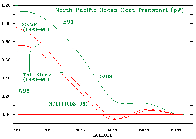
Figure 2. Estimates of northward heat transport from integrals of air-sea flux and from zonal hydrographic transects in the North Pacific. The air-sea flux estimates, integrated from 63°N to the latitude shown, include an estimate from the COADS climatology (Da Silva et al, 1995), plus estimates from NCEP (Kalnay et al, 1996) and ECMWF (ECMWF, 1993) operational models for the years 1993-1998. The hydrographic estimates, including error bars, are based on one-time sections at 10°N (W96 is Wijffels et al, 1996) and 24°N (B91 is Bryden et al, 1991). The estimate from the present study is also shown, 0.77 ± 0.12 pW for 1993-1998, at the equivalent latitude (See Section 5, Eq. 1) appropriate for comparison with ECMWF.

2. XBT/XCTD transects

Sampling was initiated in September 1991 on SS Sea-Land Enterprise, a container ship operating along a track from San Francisco to Taiwan via Honolulu and Guam (Fig 2). A scientist rides on the ship for the 17-day crossing approximately every three months, collecting an eddy-resolving temperature transect using Sippican Deep Blue (800 m) XBTs. About 305 temperature profiles are obtained on each voyage, with probe spacing ranging from about 10 km near the western boundary to 50 km in mid-ocean. Sampling terminates near the 200 m isobath at both endpoints, with closely spaced probes near topography. Salinity sampling with XCTD probes was begun in 1994 and about 18 XCTDs are deployed on each cruise to determine large-scale temperature/ salinity characteristics and variability. Processing of the XBT and XCTD data, including fall-rate correction and interpolation onto a uniform grid (with spacing 0.1° of longitude by 10 m depth) was described by Gilson et al (1998). Geostrophic velocity was calculated from gridded specific volume, using a reference level at 800 m. The specific volume calculation uses salinity that is estimated on a cruise-by-cruise basis from XCTD profiles when available (Gilson et al, 1998).

Through January 1999, 27 XBT/XCTD transects have been completed on the Enterprise. Initial cruises were at 6-month intervals, changing to approximately 3-month intervals at the end of 1992. Here, we will consider the 25 quarterly transects from November 1992 to January 1999 as representing the period 1993-1998.

3. Wind, wind stress and Ekman transport

An anemometer (R.M. Young 5103, propeller/vane) was installed above the bridge of the Enterprise in 1995 and has operated since that time. GPS navigation is used to remove ship motion from the relative wind measurements. A second anemometer was installed near the bow on the ship's foremast in 1998, a location thought to be less subject to disturbance of the airflow by the ship's structure. The anemometer is sampled and recorded once per minute and is vector averaged to 6-hourly intervals. The 6-hourly ECMWF data are interpolated in space, using a weighted average of the adjacent nine grid points, to the instantaneous location of the Enterprise. In this and all other transects the anemometer wind speed and direction are highly correlated with ECMWF analyses.

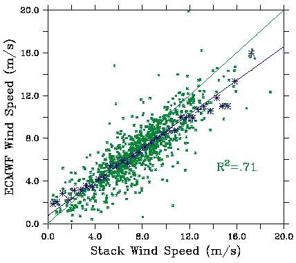
A comparison of all 6-hourly winds from the Enterprise, corrected as noted above, with the corresponding 6-hourly ECMWF winds is shown in Fig 3. The figure also shows the average ECMWF wind speed in each 0.5 m/s bin of anemometer wind speed. A systematic difference at high wind speed is clear, with ECMWF values being lower than anemometer wind by 2.6 m/s at 15 m/s wind speed. There is no systematic difference in wind direction, which is highly correlated (R2=0.89) in the two datasets. A correction based on the regression line in Fig 3 was applied to the ECMWF wind data, uniformly along track.

Wind stress is calculated from corrected ECMWF 6-hourly winds using the drag coefficient formulation of Yelland et al (1998). The details of this formulation differ from that of Large and Pond (1981). However, in the present case, the mean Ekman transport across the XBT/XCTD transect differs by only a few percent depending on which is used. The particular choice of drag coefficient between these two does not have a large impact on the calculation.

Ekman transport across the ship track is tx/rf, where tx is the component of wind stress parallel to the ship track, r is the water density, and f is the Coriolis parameter. Ekman transport estimates were computed using corrected ECMWF wind, and averaged over 1-month intervals from January 1993 to December 1998. The mean over 72 months is 15.9 ± 0.8 Sv northward. A 12-month running mean is shown in Fig 6 (red line) to illustrate the interannual variability in Ekman transport. The interannual oscillation ranges between 13 and 20 Sv with maxima in early 1994 and early 1997.

The temperature associated with Ekman transport is ambiguous since the penetration depth of the directly wind-driven flow is not known. For the present XBT dataset, we take the temperature at 5 m to represent the sea surface temperature and the temperature of the Ekman transport. A second calculation, with the Ekman layer assumed to decay linearly over the top 50 m, produced a decrease in the average temperature of the Ekman layer by 0.2°C and a decrease in the net heat transport by 0.01 pW. This difference is not significant.

Figure 3. Regression plot of bridge anemometer wind speed (6-hourly values from all transects, corrected downward by 5% for height and location bias) versus ECMWF as small green symbols. Large black symbols show average values, in bins of 0.5 m/s width of the bridge anemometer wind speed. Also shown are a line having unit slope and a line that is the best fit to the 6-hourly measurements.

4. Geostrophic transport

The 25-cruise mean geostrophic transport is 17.5 ± 0.8 Sv southward in the upper 800 m. In this transect, the northward flow of the Kuroshio, about 21.5 Sv, is over-balanced by 39.0 Sv of southward flow in the interior. Of the latter, 10.1 Sv of southward transport occurs to the east of Hawaii. The maximum net southward transport in a single cruise was 26.5 Sv in November 1998, and the minimum was 11.1 Sv, in November 1995. This large spread illustrates the potential hazard of using one-time transects as representative of the mean transport. Transport variability is described in Sections 6-7.

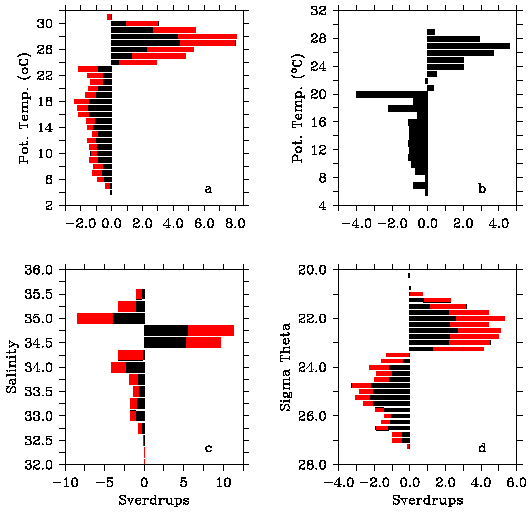
Fig 4a illustrates how the mean of geostrophic plus Ekman transport is partitioned in temperature classes. The southward geostrophic transport shows a broad maximum centered in the 17-18° band. Waters in this temperature class are the Subtropical Mode Waters (STMW) formed in both the western (15-19°C waters, e.g. Masuzawa, 1969) and eastern (16-22oC, Hautala and Roemmich, 1998) Pacific. The broad temperature range of southward transport is consistent with these STMWs plus the colder Central STMW (9-13°C) described by Suga et al (1997). Cruise-to-cruise standard deviations (Fig 4a, red bars) in the thermocline are substantial, but smaller than the mean transports. For example, combined transport in the 15-22° range is 9.0 Sv with cruise-to-cruise standard deviation of 2.7 Sv. The higher variability at warmer temperatures is primarily due to seasonally changing temperature in the surface layer rather than to changing velocity. Interestingly, the maximum southward transport in the 24°N hydrographic transect (Fig 4b) occurred at a warmer 20°C, presumably another artifact of selecting a single realization. The contrast of Fig 4a and 7b again demonstrates the necessity of multiple realizations in order to determine the mean and variability of basin-wide geostrophic transport.

Transport in salinity classes (Fig 4c) shows northward flow concentrated around a salinity of 34.75, between two bands of southward transport. There is a strong southward maximum at 35.0, characteristic of the subtropical gyre interior. A band of fresher transport, mostly between 33.0 and 34.0 is due to the California Current system carrying waters of subpolar origin. Transport in density classes (Fig 4d) shows the same pattern as Fig 4a, indicative of the strong control of density by temperature at these latitudes. The thermal overturning circulation carries heat and buoyancy northward, while the transport of freshwater appears small.

Figure 4. a. Geostrophic plus Ekman transport in 1°C temperature bins. Black bars show the mean values from 25 cruises. The width of the red bar beyond the end of the black bar is the standard deviation. b. Geostrophic plus Ekman transport from the one-time hydrographic transect at 24°N (Bryden et al, 1991). c. Same as a) but for salinity bins. d. Same as a) but for density bins of sigma-theta.

The volume transport (Fig 4) includes both the gyre-scale parts of that field and components due to boundary currents and eddies. The characteristic structure and transport of eddies, including their interannual variability, is the subject of a separate study (Roemmich and Gilson, 1999).

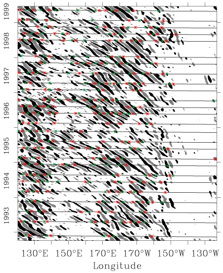
Fig 9 (from that work) shows eddy locations identified independently in the T/P and XBT datasets. The coincidence of features in the two datasets is remarkable. The T/P dataset allows individual eddies in the XBT cruises to be clearly tracked for a year or longer. In that time, they move thousands of kilometers to the west at about 10 cm/s. It is the diagonal nature of the ship track (Fig 1) toward Guam and Taiwan that limits the ability to follow individual features even farther westward. A separate map of T/P height along constant latitude of 22°N (not shown) demonstrates that individual features can be tracked continuously from near Hawaii to the western boundary. In Fig 9, the decrease in eddies near 150° E is clearly associated with the southward dip of the ship track toward Guam, away from the eddy-rich latitudes near 20°N (Fig 1).

The eddy transport is significant, enhancing the thermal overturning circulation by about 4 Sv in the mean (due to correlation of velocity anomalies with layer thickness anomalies) and accounting for a large fraction of the interannual variability in southward thermocline transport. For the present work, it suffices to say that the eddy transports are included in these calculations. They are embedded in the boundary-to-boundary integrals of the geostrophic flow and are a part of the signals described here.

5. Closure of the mean mass and heat budgets

The 1.6 Sv difference between the net northward Ekman transport and the net southward geostrophic flow could be due to random sampling errors or systematic error in the estimate of Ekman transport. If it is not one of these errors, then the additional 1.6 Sv of northward transport needed to complete the mass balance is due to barotropic transport or to deep baroclinic shear (below 800 m) not sampled by the XBTs. We will close the mass budget, assuming that the imbalance is not due to sampling errors, and then consider the additional uncertainty due to errors. With respect to estimating heat transport, the extreme possibilities are as follows:

1a) The additional 1.6 Sv of northward transport is all in the upper 800 m in the relatively warm western boundary. In other words, suppose there is mean shear in the Kuroshio just below the 800 m level. Then, the appropriate temperature for the balance is the 0-800 m average temperature, 13.9°C (120.6°E to 123.8°E)

2a) The 1.6 Sv is all in the barotropic component (3.6°C, Bryden et al, 1991). Closure of the mass balance in these two scenarios results in northward heat transport estimates of 0.80 and 0.73 pW respectively.

The above range of heat transports must be expanded to reflect the random sampling uncertainty. Again, we select the possibilities that produce the maximum range:

1b) Change scenario 1a) above by increasing the northward Ekman transport by the standard error, 0.8 Sv at 27.1°C, balanced barotropically at 3.6°C.

2b) Change scenario 2a) by decreasing Ekman transport by 0.8 Sv, again with a barotropic mass balance.

This expands the range of values to 0.88 and 0.65 pW respectively. We choose the central value as the best estimate, hence, Mean meridional heat transport = 0.77 ± 0.12 pW. This uncertainty does not include the possibility of systematic errors in the wind field, which are discussed in Section 8.

The estimate given above, 0.77pW ± 0.12, is for ocean heat transport across the XBT transect. For comparison with other techniques, it is desirable to give an estimate of heat transport across a constant latitude. To do this, we define an "equivalent latitude", YE, across which the heat transport is the same as it is across the XBT track. YE is about 18ýN for the ECMWF (1993-1998) values of QNET, 20°N for NCEP (1993-1998), and 22°N for the COADS climatology of DaSilva et al, 1995. In Fig 1, the present estimate is plotted at the ECMWF equivalent latitude, where it is in very good agreement with the ECMWF air-sea heat flux integral. By shifting the estimate to 20°N or 22°N, it is seen to be slightly inconsistent with the NCEP and COADS values.

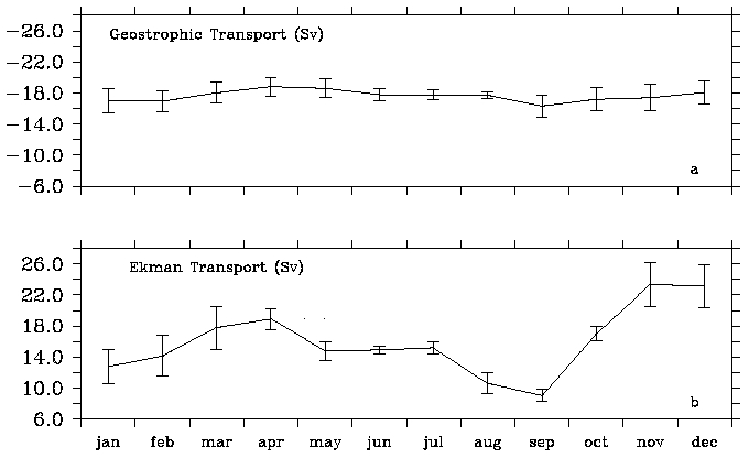
6. Seasonal variability

The annual cycles of geostrophic and Ekman transport are shown in Fig 5.

For the geostrophic component (Fig 5a), accurate averages for every month cannot be obtained because of the small number of cruises. With 25 cruises, there are only about two in a given month. We therefore averaged cruises in a given month with those of the month before and after. Thus, Fig 5a shows 3-month running averages based on about six cruises each. It is apparent that none of the estimates is significantly different from the mean and that there is not a large annual cycle in geostrophic transport.

Ekman transport (Fig 5b) shows a semi-annual behavior, with maxima in April and November and minima in January and September. Here the means and standard errors for each month are based on the six monthly average values for a given month during 1993-1998. Wind variability is large, so the annual cycle is not accurately determined from the 6-year dataset. However, climatological data (Hellerman and Rosenstein, 1983) examined along this track show a similar semi-annual pattern, amplitude, and phase, so the 6-year interval is thought to be representative.

The absence of an annual cycle in baroclinic transport implies that the mass balance for the annually varying Ekman transport is accomplished through barotropic waves. This is not surprising, and is consistent with evidence from TOPEX/Poseidon altimetric data. Baroclinic waves are seen to propagate westward from Hawaii to Taiwan in a period of about 2 years (Chelton and Schlax, 1996, Roemmich and Gilson, 1999). Adjustment of baroclinic transport to changes in basin-wide wind forcing is expected on interannual but not annual time-scales.

Figure 5. Annual cycle of geostrophic and Ekman transports. a. The mean and standard error of geostrophic transport using all cruises in a sliding 3-month window (e.g. all cruises in Dec-Jan-Feb from any year, Dec 1992 - Jan 1999 for the Jan estimate) b. The mean and standard error of Ekman transport, from corrected (see text) ECMWF values. The Jan value is the mean of all Jan data 1993-1998, etc.

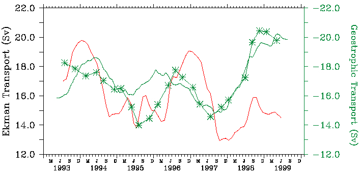
7. Interannual variability

The interannual pattern of Ekman transport (red line in Fig 6, the 12-month running mean) is plotted together with the corresponding time-series of geostrophic transport. The interannual geostrophic transport time-series is obtained by applying a 4-cruise running mean to the transport from individual cruises. The geostrophic and Ekman transports have interannual fluctuations that are similar to one another but of opposite sign. There is an approximate balance between northward Ekman transport and southward geostrophic transport, with an oscillation period of about 3 years. There is also a suggestion of a trend in geostrophic transport toward greater southward values and in Ekman transport toward weaker northward ones.

Figure 6. Interannual variability of geostrophic and Ekman transports. Northward Ekman transport is the 12-month running mean (red line). Southward geostrophic transport is the 4-cruise running mean (solid line and symbols). Southward geostrophic transport from TOPEX/Poseidon is shown as the green line.

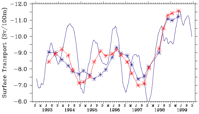
The time-series of geostrophic transport is based on quarterly XBT/XCTD cruises (Fig 6), so an important question is whether this time-series is badly aliased by unresolved high frequency variability. As a test, geostrophic transport variability at the sea surface from the XBT/XCTD cruises is compared to the same quantity derived from 10-day cycles of TOPEX/Poseidon altimetric data interpolated onto the ship track (Gilson et al, 1998). Fig 7 compares XBT/XCTD-derived surface geostrophic transport (black line), with TOPEX/Poseidon surface geostrophic transport (blue and red lines), The mean transport cannot be determined from TOPEX/Poseidon, so that series is adjusted to have the same mean as the XBT/XCTD series. The two measures of interannual variability in surface geostrophic transport in Fig 7 show a similar 3-year oscillation to the total geostrophic transport (Fig 6). At the times when the two surface transport estimates are most different (e.g. mid-1994), inspection of the datasets shows that the differences are due to Kuroshio transport variability close to the western boundary rather than to temporal aliasing. This transport variability is not adequately observed by TOPEX/Poseidon because there are no good altimetric data close to the inshore side of the current at this location. In addition, if the TOPEX/Poseidon surface transport time-series is smoothed with a 360-day running mean (not shown), it is very similar to the sub-sampled version (red line in Fig 7). It is therefore concluded that the interannual time-series of total geostrophic transport (Fig 6) is not badly distorted by aliasing. The similarity of geostrophic transport to Ekman transport is not simply a coincidence between heavily filtered and noisy datasets.

Fig 7 also indicates that there is an annual cycle in the surface geostrophic transport. The TOPEX/Poseidon series, smoothed by a running mean of 120 days, shows 6 peaks, one around January of each year. This is in contrast to Fig 5, where an annual cycle was not detected in total (0-800 m) geostrophic transport from XBT/XCTD data. The explanation of this disparity is that the annual cycle is confined to depths above 100 m. It is detectable in surface geostrophic transport from the XBT/XCTD data but not in the 0-800 m integrated transport.

Figure 7. Comparison of geostrophic surface transport from XBT/XCTD transects (solid line, 4-cruise running mean) with TOPEX/Poseidon geostrophic surface transport. (The blue line is the 120-day running mean from the complete T/P dataset. The red line with symbols is sampled at the time of the XBT/XCTD cruises, then subject to a 4-cruise running mean). The symbols mark the cruise times.

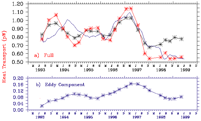
The interannual time-series of Ekman and geostrophic transports (Fig 6) are used to estimate heat transport (Fig 8a). At the time of each cruise, the residual mass field (difference between northward Ekman and southward geostrophic transport, filtered as in Fig 8a) is balanced in two different ways, similarly to the time mean calculation in Section 5. One balance assumes barotropic compensation at 3.6°C (red line), and the other assumes that the balancing transport occurs in the upper 800 m in the western boundary current, at an average temperature of 13.9°C (solid line). These two possibilities for the unmeasured deep fields produce the greatest range in heat transport. It is clear that interannual heat transport variability is substantial, with changes on the order of 0.3 pW. The heat transport pattern (Fig 8a) roughly follows that of Ekman and geostrophic transport (Fig 6). It is modulated by variability in the temperature of the Ekman layer and in the vertical structure of the geostrophic transport profile, and importantly, by changes in the eddy transport (v'T'). The interannual variability in eddy heat transport, from Roemmich and Gilson (1999), is shown in Fig 8b. Its range is about 0.1 pW, a substantial fraction of the total interannual heat transport variability. Moreover, the upward trend in eddy heat transport tends to balance a decrease due to diminishing Ekman transport (Fig 6) so that the total (Fig 8a) does not show a trend.

What is the significance of interannual anomalies in ocean heat transport of order 0.3 pW? This can be addressed in a couple of different ways. First, it amounts to a substantial modification of the meridional overturning circulation depicted in Fig 4. The amplitude of this circulation changes by more than 30% on interannual periods. Second, because the area of the North Pacific to the north of the XBT/XCTD transect is about 3.6 x 1013 m2, the anomalous heat transport amounts to nearly 10 w/m2 on average over the whole of this area. This heating is undoubtedly distributed unevenly over the basin, so it can be quite significant regionally - to cause anomalous warming or cooling and possibly feedback to the atmosphere. Unlike the annual cycle variability, which we argued is not highly significant because of the short displacement of water parcels over a few months, the interannual anomalies penetrate thousands of kilometers even at interior ocean velocities.

Figure 8. a. Time-series of interannual variability in northward heat transport. The three lines are for the barotropic (red line) and baroclinic (solid line) mass closure schemes described in the text. The blue line is northward heat transport as inferred from ECMWF heat fluxes integrated over the ocean surface north of the XBT section. b. Interannual variability in eddy heat transport (from Roemmich and Gilson, 1999), smoothed by 4-cruise running mean.

Figure 9. Eddy locations in T/P and XBT data as a function of longitude and time. Warm (cold) core eddies with sea surface height maxima (minima) are shown as red (green) symbols for XBT data and gray (black) shading for T/P data.

8. Discussion and conclusions

In the present work, the value of regularly repeating measurements of the upper-ocean temperature and geostrophic shear fields has been demonstrated. The mean of geostrophic transport in the upper 800 m, 17.5 ± 0.8 Sv southward during 1993-1998, is well determined by the time-series of 25 cruises. This approximately balances the Ekman transport, 15.9 ± 0.8 Sv northward for the same 6-year period. The heat engine of the North Pacific consists of northward Ekman transport of warm surface water plus northward geostrophic transport in the warm Kuroshio. The balancing southward geostrophic flows in the ocean interior occur at a broad range of thermocline temperatures centered on 17-18°C Subtropical Mode Waters (Fig 4). This is the shallow meridional overturning circulation of the subtropical North Pacific. Moreover, the 6-year time-series demonstrates that geostrophic and Ekman transports remain in approximate balance on interannual periods, while the amplitude of the overturning circulation varies by over 30% (Fig 6).

The mean northward heat transport is 0.77 ± 0.12 pW across the XBT/XCTD transect, which crosses the North Pacific at an average latitude of 22°N (Fig 1). The error bounds on this estimate result from uncertainty in balancing the 1.6 Sv difference between northward Ekman and southward geostrophic flows and from random sampling errors in the 25-cruise, 6-year time series. Systematic errors in the wind field have been addressed (Fig 3) but may still be significant, and are not included in the error bounds.

It is interesting to note that the error bounds on heat transport assigned to the one-time hydrographic surveys at 24°N and 10°N (Fig 2) span a wide range of values including both the climatological estimate and the operational model estimates for 1993-1998. The present study finds good agreement with the net air-sea heat flux integral from ECMWF (Fig 2) but the lower error bounds marginally exclude the estimates from NCEP and the COADS climatology. This result is for a single region, so it should not be taken as a general confirmation or correction of the flux products. However, it illustrates the potentially powerful use of the oceanic heat transport estimates for constraining or testing models (e.g. Wilkin et al, 1995) and operational analyses. Moreover, it clearly emphasizes the high premium attached to accurate determination of the wind field. Errors in the wind field affect both air-sea flux estimates (via latent heat exchange) and the oceanic heat transport (via the Ekman layer).

Interannual variability in ocean heat transport was found to be of order 0.3 pW (Fig 8a) - amounting to nearly 10 w/m2 of anomalous heating/cooling over all of the North Pacific to the north of this transect. This finding highlights the need to close the time-varying heat budget including air-sea fluxes and storage, with errors less than 10 w/m2 on interannual time-scales. This will reveal the patterns of coupled variability in the air-sea system and bring into focus the role of ocean circulation as a potential feedback mechanism. For now, the similarity of geostrophic and Ekman transport variability on interannual time-scales demonstrates that this climatically significant variability in ocean circulation can be measured and tracked.

Acknowledgements

Collection of the XBT/XCTD data was supported by the National Science Foundation through Grants OCE90-04230 and OCE96-32983 as part of the World Ocean Circulation Experiment. TOPEX/Poseidon data were kindly provided by the Jet Propulsion Laboratory, and the assistance of L.-L. Fu and A. Hiyashi is gratefully acknowledged. Analysis was supported by the NASA JASON-1 project through JPL Contract 961424. We are grateful for the dedicated efforts of many ship riders in collecting the XBT/XCTD data, under the management of G. Pezzoli. The development and production of VOS IMET modules has been carried out by D. Hosom and is supported by NOAA Grant NA47GP0188 (JIMO Consortium). The views expressed herein are the authors' and do not necessarily reflect those of NOAA or its sub-agencies. We thank the officers and crew of SS Sea-Land Enterprise for their continued assistance to this project. Chief Mate M. Smith provided invaluable programming support in the installation of the anemometers on the Enterprise. The National Center for Atmospheric Research provided access to ECMWF analysis products. Graphics were produced using FERRET, developed by NOAA/PMEL.

References

Bennett, A. and W. White, 1986: Eddy heat flux in the subtropical North Pacific. J. Phys. Oceanogr., 16, 728-740.

Bryden, H., D. Roemmich and J. Church, Ocean heat transport across 24oN in the Pacific. Deep-Sea Res., 38. 297-324, 1991.

Chelton, D. and M. Schlax, Global observations of oceanic Rossby waves. Science. 272, 234-238, 1996.

DaSilva, A., C. Young and S. Levitus, Atlas of Surface Marine Data 1994, vol. 1, Algorithms and Procedures. NOAA Atlas NESDIS 6, 83 pp., Natl. Oceanogr. Data Cent, Silver Spring, Md., 1995.

European Centre for Medium-Range Weather Forecasts (ECMWF), The description of the ECMWF/WCRP III - A global atmospheric data archive. Tech. Attachment ECMWF 1-18, Reading, England, 1993.

Freilich, M. and R. Dunbar, The accuracy of the NSCAT 1 vector winds: Comparisons with National Data Buoy Center buoys. J. Geophys. Res., in press, 1999.

Gilson, J., D. Roemmich, B. Cornuelle and L.-L. Fu, Relationship of TOPEX/Poseidon altimetric height to steric height and circulation in the North Pacific. J. Geophys. Res., 103, 27947-27965, 1998.

Hautala, S. and D. Roemmich, Subtropical mode water in the Northeast Pacific Basin. J. Geophys. Res., 103, 13055-13066, 1998.

Hellerman, S. and M. Rosenstein, Normal monthly wind stress over the World Ocean with error estimates. J. Phys. Oceanogr., 13, 1093-1104, 1983.

Hsu, S., E. Meindl and D. Gilhousen, Determining the power-law wind-profile exponent under near-neutral stability conditions at sea. J. Applied Met., 33, 757-765, 1994.

Kalnay, E., M. Kanamitsu, R. Kistler, W. Collins and 18 others, The NCEP/NCAR 40-year reanalysis project. Bulletin of the American Meteorological Society, 77, 437-471, 1996.

Large, W. and S. Pond, Open ocean flux measurements in moderate to strong winds. J. Phys. Oceanogr., 11, 324-336, 1981.

Macdonald, A. and C. Wunsch, An estimate of global ocean circulation and heat fluxes. Nature, 382, 436-439, 1996.

Masuzawa, J., Subtropical mode water. Deep-Sea Res., 16, 463-472, 1969.

Roemmich, D. and J. Gilson, Eddy transport of heat and thermocline waters in the North Pacific: A key to interannual/decadal variability. Submitted to J. Phys. Oceanogr., 1999.

Roemmich, D. and T. McCallister, Large scale circulation of the North Pacific Ocean. Prog. Oceanogr., 22, 171-204, 1989.

Stephens, G., G. Campbell, and T. Vonder Haar, Earth radiation budgets. J. Geophys. Res., 86, 9739-9760, 1981.

Suga, T., Y. Takei and K. Hanawa, Thermostad distribution in the North Pacific subtropical gyre: the central mode water and the subtropical mode water. J. Phys. Oceanogr., 27, 140-152, 1997.

Trenberth, K. and A. Solomon, The global heat balance - heat transports in the atmosphere and ocean. Climate Dynamics, 10, 107-134, 1994.

Weller, R. A. and S. P. Anderson, Surface meteorology and air-sea fluxes in the western equatorial Pacific warm pool during the TOGA Coupled Ocean-Atmosphere Response Experiment, J. Climate, 9(8), 1959-1990, 1996.

Weller, R. A., M. F. Baumgartner, S. A. Josey, A.S. Fischer, and J. C. Kindle, Atmospheric forcing in the Arabian Sea during 1994-1995: observations and comparisons with climatology and models, Deep-Sea Research, 45(11), 1961-1999, 1998.

Wijffels, S., E. Firing and H. Bryden, Direct observations of the Ekman balance at 10-degrees-N in the Pacific. J. Phys. Oceanogr., 24, 1666-1679, 1994.

Wijffels, S., J. Toole, H. Bryden, R. Fine, W. Jenkins and J. Bullister, The water masses and circulation at 10oN in the Pacific. Deep-Sea Res., 43, 501-544, 1996.

Wilkin, J., J. Mansbridge and J.S. Godfrey, Pacific Ocean heat transport at 24oN in a high-resolution global model. J. Phys. Oceanogr., 25, 2204 - 2214, 1995.

Yelland, M., B. Moat, P. Taylor, R. Pascal, J. Hutchings and V. Cornell, Wind stress measurements from the open ocean corrected for airflow distortion by the ship. J. Phys. Oceanogr., 28, 1511-1526, 1998.